10. Causal Discovery to Null Variable Dataset

Now that we have a Knowledge Box with what seems a reasonable set of constraints (edges cannot form from variables in the next time period into variables in the current time period), we conduct our search.

10.1 Apply Causal Discovery (Bootstrapped Search) to the Dataset Expanded with Null Variables

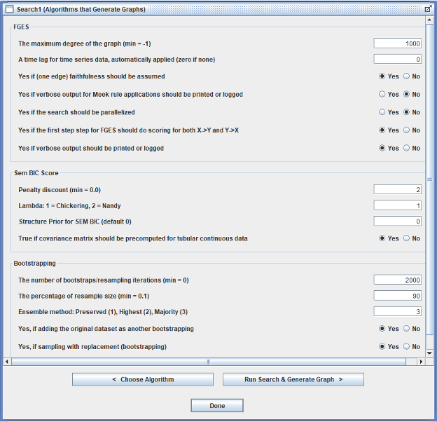
The settings in the Search box are set as follows, which generally are the same as for our pre-null variable-injected search but this time performed on the 175-variable and 5414-case dataset:

• Knowledge box:
  • We utilized the knowledge box presented in the previous subsection to help ensure that the edges formed have reasonable or at least not unreasonable orientations
• Algorithm: Fast Greedy Equivalent Search (FGES)
• Score method: Structural Equation Modelling Bayesian Information Criterion (SEMBIC)
• Penalty Discount: 2 rather than the usual default 1
  • Results in a sparser graph than the default setting of 1, reducing the number of false-positive edges (at the cost of more missing, that is, false-negative, edges; but that are also weaker in cause-effect)
• Symmetric First Step: set to Yes
• Faithfulness:
  • In the Tetrad GUI, this setting is labelled this way:
    • “Yes if (one edge) faithfulness should be assumed”
• Number of Bootstraps = 2000
  • We use a larger number of bootstrap samples to improve precision and replicability of search results
  • Because the search setting “Include the original dataset as an additional bootstrap sample” is set by default, there will actually be 1001 bootstrap samples searched, an odd number, which is relevant to interpreting the result from the Majority Ensemble Method setting
• Percentage of Resample Size = 90
• Ensemble Method: Majority (2 or 3)
  • An edge is kept only if it appears in the majority of bootstrap sample search results in other words, if it appears in at least 501 of the 1001 searches.
• Otherwise, use default settings for the search

Below is a screenshot of the second menu window for search hyperparameter settings (Tetrad version 7.1.2-2). (We don’t show the first menu window settings as the settings are identical to that for the initial screen; and note that the second menu window differs from that of the initial screening’s second menu window in only one setting: the number of bootstrap samples is 2000 instead of 10.)

Applying causal discovery to the 175-variable dataset produces a busy search graph, but we can display the graph, one portion (subgraph) at a time to get a better sense of what’s going on. We use the Graph box Display Subgraphs feature of the Tetrad GUI to focus only on a group of variables of interest at a time, selecting a group of variables and then selecting “Adjacents” to display which variables are adjacent to the members of the group (i.e., either have an edge going into a member of the group or are a destination of an edge coming out of a member of the group). We do this selection/display process in stages:

• Null Variables and their adjacencies
• Remove all variables not adjacent to Start or one of the 18 sociotechnical and work-rate variables or Start
• The binarized variables causally-adjacent to the 18 sociotechnical and work-rate variables or Start
• The 19 sociotechnical, work-rate, and Start variables as a Causal Subgraph

The null variables and their adjacencies

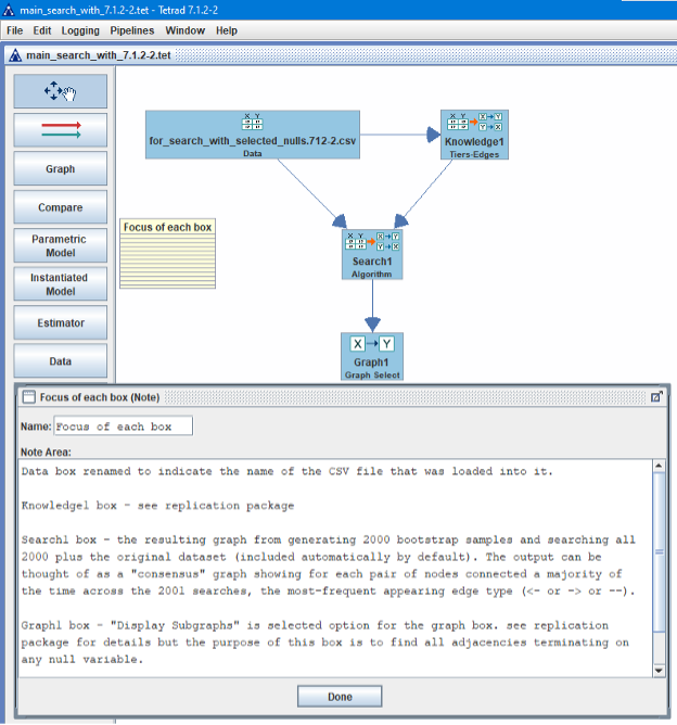
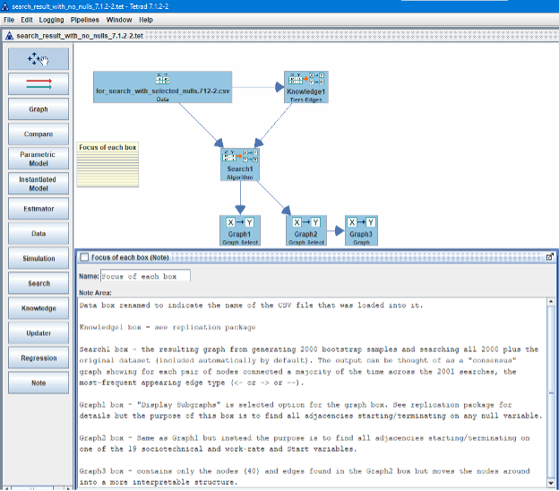
We hang a graph box Graph1 under the Search box as shown below (we also added a note to briefly explain each box) to begin this process of exploring particular subsets of variables:

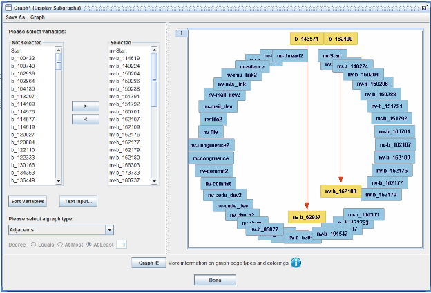
Opening the Graph1 box, we declare it The vertical “Selected” list only shows 20 of the 42 null variables, but all 42 appear in the scrollable list. Then “Adjacents” is selected from the pull-down menu under “Please select a graph type.” Then “Graph It!” was clicked on which produced a blank graphic panel, but that’s because the null variables appear far far to the right of the graphic panel and you need to scroll right using the scroll control under the graphic panel to see them. Clicking anywhere in the white space of the graphic panel, bring up the context menu and select “Circle.” A total of only 2 edges for these 42 variables appear! They are with two of the non-null-variable binarized variables (and one of them matches its binarized counterpart, which rarely happens): nv-b_62937 <– b_143571 and nv-b_162180 <– b_162180. There are no others! The null variables, which in theory will be, on average at best very weakly correlated with any other variables, fail to form edges with any other variables—even themselves—except on two occasions a majority of the time when conducting bootstrapped search.

If we had encountered many adjacencies terminating on the null variables, it could indicate: (1) there was a problem in the pseudo-random number generation (or the way we set it up) of not generating numbers with sufficient independence, (2) our dataset is too small to reduce the incidence of not-so-very-weak correlations of null variables with non-null variables, and/or (3) our penalty discount was insufficiently high thereby allowing false-positive adjacencies to arise, and if they arise among the null variables with known statistical properties (apparent independence from all other variables), then it would imply that some or even many of the adjacencies that arise among the binarized variables, current time-period variables, and next time-period variables are also false positives. Fortunately, with only two adjacencies, we can go forward with more confidence. (Remembering, though, that confounders, such as the idiosyncratic attributes of a particular person, or their training, might create correlations among variables both within and across time periods that might lead causal discovery to impute adjacencies where there should be none. There is of course, never a perfect dataset for any analysis and shortcomings of any analysis that might be performed. In Causal Inference with observational data, we become aware of how such confounding can be an “Achilles Heel” but of course, confounding likewise impacts the results of non-causal-based statistical analyses such as linear or logistic regression, though this limitation is often underappreciated.

And here is a copy of the Tetrad session so far:

+ main_search_with_7.1.2-2.tet

Remove all variables not adjacent to Start or one of the 18 sociotechnical and work-rate variables or Start

Using a similar technique we can, first, create a Graph2 box to display only the variables adjacent to Start and 18 sociotechnical and work-rate variables; and second, hang off a Graph3 box off of Graph2 (select “Graph” from the pull-down menu rather than “Display Subgraphs” as we did for Graph1 and Graph2) to inherit the result of the display. Here’s the result of doing the work in the Graph2 box (and then we’ll discuss the Graph3 box):

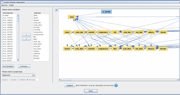
Note the scroll control under the pane holding the graph. We click on “Done” and then add the Graph3 box with an arrow from Graph2 into Graph3 and selecting “Graph” as mentioned when creating Graph3. We’ll see something like this:

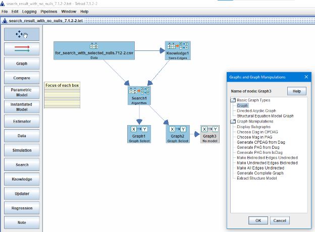
And then clicking “OK” and opening the Graph3 box, we now have the set of variables we’re interested in making a compact graph out of. The next step is highly manual—we drag the sociotechnical and work-rate variables toward the center; place parent binarized variables on their left and children binarized variables to their right; and the Start variable goes under the 18 sociotechnical and work-rate variables. Here’s the starting point (note this is identical to what we’d see in the Graph2 box at this point):

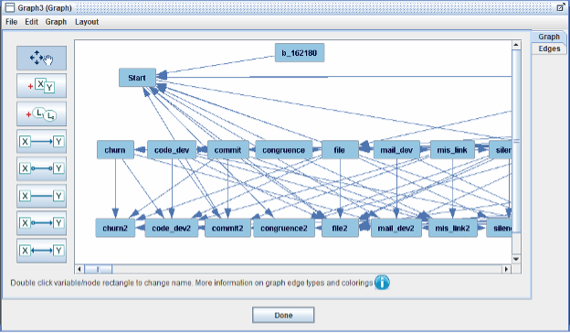
Selecting “Graph” in the ribbon and then “Graph Properties” we’ll see that there are 40 nodes meaning 21 (=40-18-1) binarized variables (b_*) that have at least one edge into one or more of the sociotechnical and work-rate variables And the ending point:

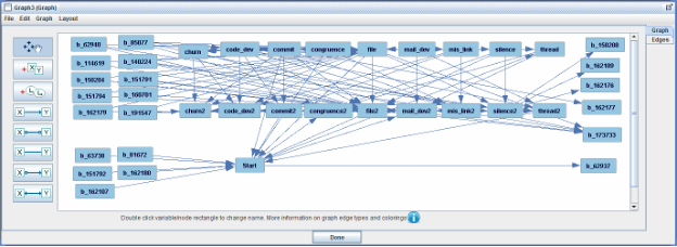
15 binarized variables are parents and 6 are children of the 19 sociotechnical and work-rate and Start variables. Here’s what the overall Tetrad session looks like:

And here’s the file with a copy of the above Tetrad session:

+ adjacents_to_the_19_7.1.2-2.tet

The binarized variables causally-adjacent to the 18 sociotechnical and work-rate variables or Start

First, we repeat the graph from the 10-bootstrap causal search (“initial screen”) followed by the 2000-bootstrap causal search. Note that the two searches identified nearly the same set of binarized variables adjacent to “the 19” (18 sociotechnical and work-rate variables plus Start variable) in spite of their employing very different counts in bootstrap samples (10 vs. 2000).

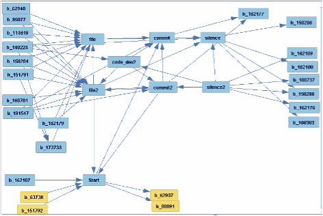
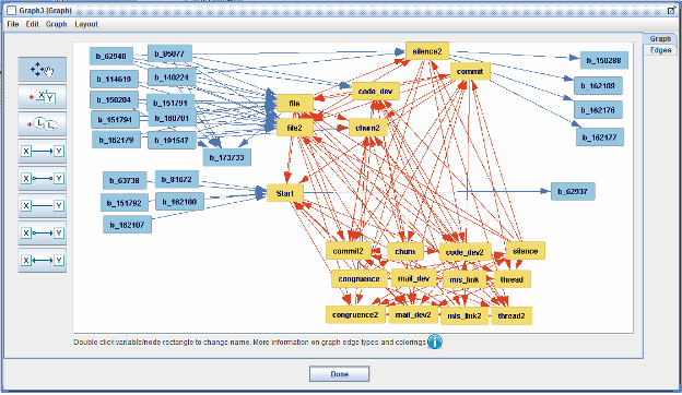
We have grouped/placed the nodes of the main-search (2000 bootstraps) causal graph (screenshot immediately above) into a layout to facilitate textual navigation:

(1) The 16 Binarized variables that are parents of one of the 19 appear on the left; 5 children on the far right; the exception being b_173733, which is the only binarized variable of 21 that is both a parent and a child. In the center, in gold, are “the 19.” The structure is relatively clean. As noted earlier, the other 114-21 CVE id variables don’t add much that’s unique and thus notable from a causal perspective. Effectively, the above causal graph is the search result. Interpretation: in general, the process that produces a CVE and remediates it is quite general across CVEs as seen by the missing 114-21 binarized variables. The initial screen produces a relatively similar set of nodes but has two additional binarized variables (23 vs. 21). (2) The 3 rows of 4 columns of socio-technical and work-rate variables at the bottom of the graph are not adjacent to any binarized variable—and thus no binarized variable has any direct causal influence on any of these 12 variables (of course there are indirect causal effects from a binarized variable to one of these 12 mediated by another variable; for example, b_62940 -> code_dev -> commit2); only the remaining 7 of “the 19” have such adjacencies and 6 appear near the top center of the pane; and Start in center left. The 6 are these: file, file2, commit, code_dev, churn2, silence2. Interpretation: these 7 (6 + Start) of the 19 are affected sometimes idiosyncratically by the CVE, but otherwise the casual graph is fairly homogenous suggesting a causal pattern that is generalizable across open-source software developments with similar features to OpenSSL during those roughly two decades that the scraped dataset represents (which features of OpenSSL matter to broader generalization are not known without further causal investigation).

We did not retain the particular layout in the last screenshot above as it was derived from an earlier screenshot just by rearranging the nodes. Having now examined generalizability, we now focus specifically on “the 19.”

10.2 Only the 19

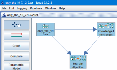
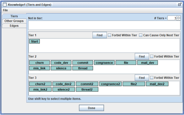
We now repeat an application of casual discovery but only for “the 19”, which means we delete all variables from the dataset except for Start, the 9 sociotechnical and work-rate variables for the current time period, and the 9 sociotechnical and work-rate variables for the next time period. These operations can be done either within or of course outside Tetrad but the resulting dataset (still 5414 rows but now only 19 columns) is found in the Data box (renamed “only_the_19”) in the screenshot below. The search settings used are the same as for the main search. The knowledge box used is the second screenshot below, which is consistent with the one used for the larger number of variables except we move Start into a tier by itself before the current time period variables (now, Tier 2) and the next time period variables (now, Tier 3). The reason is simple: force edges out of Start thereby accounting for any confounding effects it has on the rest of “the 19” and allowing us to look more directly at their causal interrelationships.

Alternatively, we could have simply trimmed the main-search-result causal graph down to just “the 19” nodes but we’re aiming for a general causal graph and would like to remove CVE-based idiosyncratic effects and instead focus on the broader casual story. And that’s why we repeated the main search with just “the 19.” The search is only about 5 minutes (vs. 60-90 minutes for the fuller search). Given the generalizability implied by the earlier analysis, the result shouldn’t be too misleading.

Here’s what the Tetrad session looks like:

And the Knowledge box:

And here is the search result, after moving some nodes around in order to mimic the layout used for Figure 9 in the article (to allow a high-level comparison):

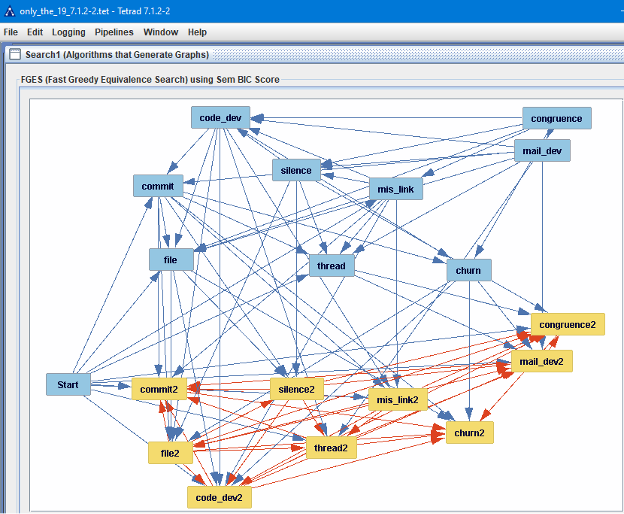
We will discuss this some more in the next subsection but a simple comparison with the original study Figure 9 shows much in common but some not in common. And here is the Tetrad session file showing the dataset, the above knowledge box, and the search result:

+ only_the_19_7.1.2-2.tet