8. Determining Which Null Features to Add Prior to Bootstrapped Search
8.1 Null Features
Null features are introduced into a dataset prior to bootstrapped search in order to determine the impact that spurious correlations have on the formation of casual edges. To calibrate the dataset to “subtract” the influence of such spurious correlations, we introduce independently pseudo-randomized versions of each feature in the original dataset (“null features”) into the dataset and record how often edges form between each pair of variables in the combined dataset during bootstrapped search. Edges that form between a pair of original features more frequently, say, than 95% of the edges that form between a null feature and any other feature in the dataset can be kept but all other edges should be dropped from the graph [1,2]. In this way, we only report those edges that are much more likely to reflect true causal associations and not spurious correlations.
When a dataset has only a few features, it is easy to create one null feature for each existing feature; however, with 133 features, a bootstrapped search could become prohibitively time expensive, including its results interpretation. Therefore, we will generate null features for only a subset of the original features. But which subset? Taking inventory of our features, we have 133 features:
- Start feature (the date when a time period started)
- Set of 9 sociotechnical and output features for the current time period
- Set of 9 features for the next time period
- Set of 114 binarized features (id-of-the-CVE-timeline indicator features)
We will create a null feature for each of the first 19 features but only a small selection of the 114 binarized features.
First, we conduct an initial screen to divide CVEs into two subsets: (1) those CVEs that seem to have no notable causally idiosyncratic role (their causal relationship to socio-technical features and worker-rate features seems about the same as most other CVEs)—for such features we won’t bother to generate a null feature as there’s perhaps nothing too unique going on that’s notably different from any other CVE from a causal perspective and thus not much to be gained from creating a corresponding null feature; and (2) those CVEs that do seem to be causally interesting and different from the others.
Toward splitting the CVEs in the above-described way, we perform an initial screen. This initial screening will also involve bootstrapping but here the intent is just to give multiple chances for a causal edge to appear with the binarized (CVE id) feature representing that CVE. For example, we might perform Causal Discovery with bootstrapping set to just 10 samples, and then drop any feature that fails to have any edge whatsoever in this quick search across 10 samples. Before presenting the results of this, we backup to discuss the tool being used for bootstrapped search.
8.2. Tetrad
To facilitate causal discovery (also known as “search”) throughout, we employed the Tetrad tool maintained at Carnegie Mellon University and the University of Pittsburgh. Various resources provide detailed descriptions of the tool and various features and algorithms, including these:
- https://sites.google.com/view/tetradcausal
- https://www.ccd.pitt.edu
- http://cmu-phil.github.io/tetrad/manual/
The final resource listed above, the Tetrad User Manual, is particularly detailed about how to use the Tetrad user interface, load a dataset, specify knowledge, run the algorithms, and import in (export out) a graph.
From a replication perspective, Tetrad can be challenging to use because often there’s no upward compatibility and later releases of the Java Runtime Environment (JRE) sometimes deprecate features of earlier releases on which an earlier release of Tetrad depends and so by the time an article is published, the replication package may no longer work as described. The solution is to indicate not only which version of Tetrad but along with it which version of the Java Runtime Environment (JRE) is needed to open a previously-saved session of Tetrad that is part of a replication package. So, in this replication package we include characterizations of both the Tetrad JAR file to use and JRE to use:
- Tetrad 7.1.2-2 release
- Last modified:
Wed Jun 08 23:54:41 UTC 2022
- Last modified:
- If the aforementioned Jar is not available, the repository with that JAR file is:
Index of /repositories/releases/io/github/cmu-phil/tetrad-gui/7.1.2-2 (sonatype.org)
- Java Runtime Environment version: Java(TM) SE Runtime Environment (build 18+36-2087)
- (More completely: Java HotSpot(TM) 64-Bit Server VM (build 18+36-2087, mixed mode, sharing)
- If that also fails, the hash for the last commit for Tetrad 7.1.2-2 release:
- https://github.com/cmu-phil/tetrad/commit/13b64f5334c4ceea5c497f675421cdb93b1c5fec
The reader may choose to replicate the analyses that follow, forgoing the provided Tetrad sessions that accompany this replication package but rather rebuild a session themselves with whatever version of Tetrad they please, and that, in general, should be fine. Of course, while results should be comparable, it’s possible that something material might have changed between versions of Tetrad or JRE releases. For this reason, we’ve tried to thoroughly specify the particular hyperparameter settings and versions used of Tetrad and the JRE.
To perform the initial screen configure Tetrad as follows:
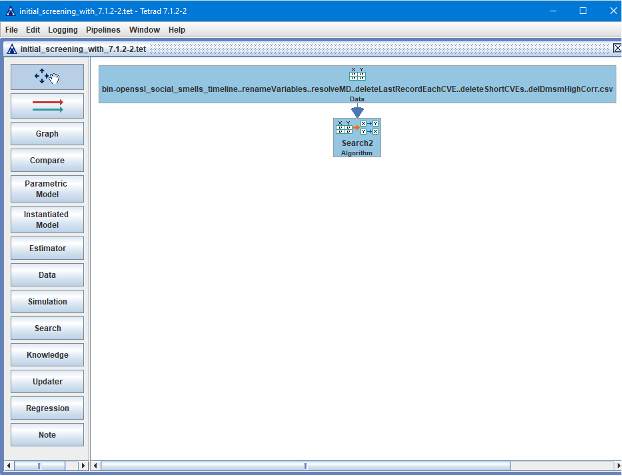
- Insert a Data box and load in the 133-variable dataset (“bin-openssl_social_smells…” – see above for full filename).
- Insert a Search box and connect the Data box to the Search box.
- No knowledge box is used for this initial application of causal discovery. Therefore, don’t be surprised if some directed edges have a reverse orientation (what should be the edge’s source appears as its target, and conversely).
- (Don’t forget you can refer to the materials hyperlinked above for how to insert the data box and search box and indeed for subsequent operations in the GUI.)
Here’s a screenshot of the initial screen Tetrad session showing the Data box on top and the Search box below that with an arrow from the Data box to the Search box. Using the context menu on the Data box, the Data box name was changed to reflect the name of the CSV file read in (which is what made the Data box so wide):

Inside the Search box, configure the search as follows:
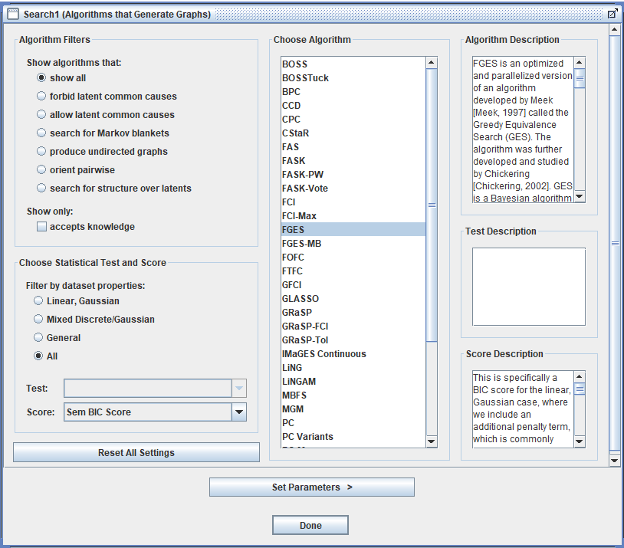
- Algorithm: Fast Greedy Equivalent Search (FGES) – one of the most written-about causal discovery algorithms with good precision (especially for determining whether there might be a direct causal relationship between two variables in the dataset; less so the orientation of that relationship: which is cause and which is effect) and speed.
- Score method: Structural Equation Modelling Bayesian Information Criterion (SEMBIC)
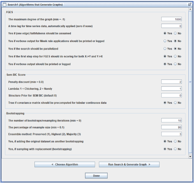
- Penalty Discount: 2 rather than the frequently-used default 1
- Given the large number of cases (our dataset has over 5000 cases), we chose to be more conservative regarding which binarized variables to include
- A higher penalty discount results in a sparser graph because the inclusion of an edge must sufficiently improve the current graph’s score for that inclusion to happen; a larger penalty discount reduces the size of that improvement in score, making the graph grow more slowly—and sparsely—during search.
- Symmetric First Step: set to Yes
- In the Tetrad GUI, this setting is labelled this way:
- “Yes if the first step for FGES should do scoring for both X->Y and X<-Y”
- In theory, for a larger dataset, this shouldn’t be necessary, but it only adds slightly to the compute time.
- In the Tetrad GUI, this setting is labelled this way:
- Faithfulness:
- In the Tetrad GUI, this setting is labelled this way:
- “Yes if (one edge) faithfulness should be assumed”
- In the Tetrad GUI, this setting is labelled this way:
- Number of Bootstraps = 10
- We’ll use a larger number of bootstrap samples when we care more about precision, but for this first run, 10 bootstrap samples drawn from the original dataset should be adequate to getting an approximate idea of which binarized variables are more active.
- Bootstrapped search tests the “neighborhood” of the data in the dataset for sensitivity to slightly different values
- Percentage of Resample Size = 90
- For determining how many cases each bootstrapped sample should contain relative to the full dataset
- 90% is the newer default; 100% used to be the default, and so we mention this setting to help achieve fuller replicability in case a different version of Tetrad is being used
- Ensemble Method: Majority (option 2 or 3, Tetrad release dependent)
- For determining which edges and frequency statistics to keep following a bootstrapped search; that is, an Ensemble Method is a way to consolidate the graphs that result from searching each bootstrapped sample of the original dataset.
- The Tetrad GUI says this about the Ensemble Method parameter, giving three options:
- “This parameter governs how summary graphs are generated based on graphs learned from individual bootstrap samples.
- If “Preserved”, an edge is kept and its orientation is chosen based on the highest probability.
- If “Highest”, an edge is kept the same way the preserved ensemble one does.
- If “Majority”, an edge is kept…” only if it appears in the majority of bootstrap sample search results.
- Otherwise, use default settings for the search
- A reminder that information about causal discovery (a.k.a., “search”), the Tetrad tool (Tetrad GUI), and search algorithm settings are found in the Tetrad User Manual cited above.
- One of the default settings is to include the original dataset as an n+1-th bootstrap sample, and so in our case here, there are actually 11 searches.
Here are screenshots of the search hyperparameter settings (Tetrad version 7.1.2-2, specifically tetrad-gui-7.1.2-2-launch.jar):


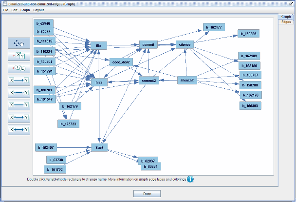
Applying causal discovery to the original dataset configured as in the above bulleted list produces a busy search graph but if we only display those binarized variables (the variables whose names match the b_* regex pattern) that have formed edges with any of the non-binarized variables in the original dataset, we obtain a simpler graph that looks something like this (after moving the variables around or even away from where the screenshot will be “snapped” so that the graph can be read more easily):

Some comments:
- Let’s examine one of these CVE variables a bit more closely: b_162107 (for CVE 2016-2107). It is for a CVE whose remediation consists of 17 consecutive time periods (the shortest possible—see subsection “Remove CVEs Whose Remediation Timeline is Too Short” above) that has a “Start” value that is near the maximum time period start for the entire dataset, indicating that it is one of the most recent CVE remediation timelines. Of course, for such a CVE, the shortness of its timeline and very high recency tell us a lot about what “Start” values to expect: among the highest ones. A correlation table shows this binarized variable to be the one with the largest correlation (positive or negative) with the Start variable. And that’s why we see this causal relationship—it simply represents the fact that for this CVE, we can predict the “Start” value pretty precisely. From the algorithmic scoring perspective, this seems to be pretty strongly causal and thus appears in the graph.
- Note that for about 10 of these depicted binarized variables, there are edges with both “file” and “file2”. These two variables (file and file2) are pretty strongly correlated (0.74), so perhaps it’s not so surprising that if the relationship between a CVE id and one of these two variables tends to form, there’s likely a strong relationship with the other variable and possibly an edge will form with it too. In contrast, the correlations between “silence” and “silence2” (correlation 0.39) and between “commit” and “commit2” (correlation 0.67) are somewhat weaker and far fewer binarized variables form edges with both members of each pair of these two variables. So, correlation is not the entire story here.
- Recall that we did not employ a knowledge box here and thus we imposed no user-defined constraints on the causal search, and thus we will not interpret the orientation of the edges in the above figure.
Here’s the Tetrad session file where the above initial screen was run and the above screenshot created:
+ initial_screening_with_7.1.2-2.tet
Having performed our initial screening that indicates which of the “b_*” variables it’s perhaps more worthwhile to create a null variable for, we move on to prepare for the main search of our entire analysis. To generate null variables, we wrote a Python program: csv-add-null.py. The program creates a copy of each variable in the dataset, randomizes the order of values within each using an appropriate pseudo-random number generator, and appends the null variable to the dataset. The program is run using Python (version 3.9) as follows:
+ python csv-add-null.py bin-dataset.csv
Where bin-dataset.csv is the output of the previous python program run.
Here is the program listing:
+ csv-add-null.v020article.py
Here is the resulting dataset, with its 266 variables (133 of them null variables) and 5414 cases (not counting the header row):
+ nv-bin-openssl_social_smells_timeline..renameVariables..resolveMD..deleteLastRecordEachCVE..deleteShortCVEs..delDmsmHighCorr.csv
Notice that in the above, we simplified the filename greatly.
[1] A. Hira, J. Alstad, and M. Konrad, “Investigating causal effects of software and systems engineering effort,” in Joint Software and IT-Cost Forum 2020.
[2] Fattaneh Jabbari, Mahdi Pakdaman Naeini, and Gregory Cooper. 2017. “Obtaining Accurate Probabilistic Causal Inference by Post-Processing Calibration.” In NIPS 2017 Workshop on Causal Inference and Machine Learning.